Assignment A01:Linear regression

Diamonds
The diamonds dataset that we will use in this application exercise consists of prices and quality information.
The variables in the diamonds dataset are
- price: price in US dollars
- carat: weight of the diamond
- cut: quality of the cut (Fair, Good, Very Good, Premium, Ideal)
- color: diamond color, from J (worst) to D (best)
- clarity: a measurement of how clear the diamond is, from I1 (worst), SI1, SI2, VS1, VS2, VVS1, VVS2, to IF (best)
Load required packages
library(QuantPsyc)## Loading required package: boot## Loading required package: MASS##
## Attaching package: 'QuantPsyc'## The following object is masked from 'package:base':
##
## normlibrary(MASS)
library(dplyr)##
## Attaching package: 'dplyr'## The following object is masked from 'package:MASS':
##
## select## The following objects are masked from 'package:stats':
##
## filter, lag## The following objects are masked from 'package:base':
##
## intersect, setdiff, setequal, unionlibrary(data.table)##
## Attaching package: 'data.table'## The following objects are masked from 'package:dplyr':
##
## between, first, lastlibrary(tidyr)
library(ggplot2)
library(GGally)## Registered S3 method overwritten by 'GGally':
## method from
## +.gg ggplot2library(gridExtra)##
## Attaching package: 'gridExtra'## The following object is masked from 'package:dplyr':
##
## combinelibrary(mosaic)## Registered S3 method overwritten by 'mosaic':
## method from
## fortify.SpatialPolygonsDataFrame ggplot2##
## The 'mosaic' package masks several functions from core packages in order to add
## additional features. The original behavior of these functions should not be affected by this.##
## Attaching package: 'mosaic'## The following object is masked from 'package:Matrix':
##
## mean## The following object is masked from 'package:ggplot2':
##
## stat## The following objects are masked from 'package:dplyr':
##
## count, do, tally## The following object is masked from 'package:boot':
##
## logit## The following objects are masked from 'package:stats':
##
## binom.test, cor, cor.test, cov, fivenum, IQR, median, prop.test,
## quantile, sd, t.test, var## The following objects are masked from 'package:base':
##
## max, mean, min, prod, range, sample, sumload data
let us check the structure of the dataset.
diamonds <- read.csv("MBA6636_SM21_Professor_Proposes_Data.csv")   #read diamonds file
head(diamonds)    #display some of the data
## Carat Colour Clarity Cut Certification Polish Symmetry Price Wholesaler
## 1 0.92 I SI2 G AGS V V 3000 1
## 2 0.92 I SI2 V AGS G G 3000 1
## 3 0.82 F SI2 I GIA X X 3004 1
## 4 0.81 G SI1 I GIA X V 3004 1
## 5 0.90 J VS2 V GIA V V 3006 1
## 6 0.87 F SI2 I AGS G V 3007 1Another function that is very useful for quickly taking a peek at a dataset is str. This function compactly displays the internal structure of an R object.
str(diamonds) #data frame by observations and variables## 'data.frame': 441 obs. of 9 variables:
## $ Carat : num 0.92 0.92 0.82 0.81 0.9 0.87 0.8 0.84 0.8 0.8 ...
## $ Colour : chr "I" "I" "F" "G" ...
## $ Clarity : chr "SI2" "SI2" "SI2" "SI1" ...
## $ Cut : chr "G" "V" "I" "I" ...
## $ Certification: chr "AGS" "AGS" "GIA" "GIA" ...
## $ Polish : chr "V" "G" "X" "X" ...
## $ Symmetry : chr "V" "G" "X" "V" ...
## $ Price : int 3000 3000 3004 3004 3006 3007 3008 3010 3012 3012 ...
## $ Wholesaler : int 1 1 1 1 1 1 1 1 1 1 ...The output above tells us that there are observations and variables in the dataset. The variable name are listed, along with their type and the first few observations of each variable.
More about the dataset
Before we go any further with the analysis, let us first understand what each column in the dataset means. And who are we going to rely on to help us with that? The American Gemological Institute (GIA). So, let’s decipher the 4Cs and other fields in the dataset.
Carat weight: Represents the weight of the diamond. Bigger, the better (if other factors are held constant).
Clarity: Refers to the absence of inclusions and blemishes. The clearer the diamond, the better the diamond, expensive the diamond (Other factors held constant).
Color: Color refers to the absence of color in diamonds.
Cut: Based on various dimensions, a diamond is assigned a cut rating or grade. This ranges from Excellent to Poor. Our dataset has the following cut ratings: Fair < Good < Very Good < Premium < Ideal Better the cut rating, expensive the diamond (other factors held constant).
Certification, polish, Symmetry, Price: These are physical dimensions of the diamond.
summary(diamonds)## Carat Colour Clarity Cut
## Min. :0.0900 Length:441 Length:441 Length:441
## 1st Qu.:0.3000 Class :character Class :character Class :character
## Median :0.8100 Mode :character Mode :character Mode :character
## Mean :0.6693
## 3rd Qu.:1.0100
## Max. :1.5800
## NA's :1
## Certification Polish Symmetry Price
## Length:441 Length:441 Length:441 Min. : 160
## Class :character Class :character Class :character 1st Qu.: 520
## Mode :character Mode :character Mode :character Median :2169
## Mean :1717
## 3rd Qu.:3012
## Max. :3145
## NA's :1
## Wholesaler
## Min. :1.000
## 1st Qu.:2.000
## Median :2.000
## Mean :2.318
## 3rd Qu.:3.000
## Max. :3.000
## NA's :1Exploring variables individually
We will investigate and visualise the distributions of the variables in this dataset. This is also referred to as univariate analysis.
First, variable classification:
- Numerical variables are classified as continuous or discrete depending on whether they can take on an infinite number of values or only non-negative whole numbers.
- If the variable is categorical, we can tell if it is ordinal by whether or not the levels are ordered naturally.
Investigating numerical data We emphasise the following points when describing the shapes of numerical distributions:
- shape:
- right-skewed, left-skewed, symmetric (skew is to the side of the longer tail)
- unimodal, bimodal, multimodal, uniform
- center: mean (mean), median (median), mode (not always useful)
- spead: range (range), standard deviation (sd), inter-quartile range (IQR)
- unusal observations
To calculate the mean, median, SD, variance, five-number summary, IQR, minimum, maximum of the price variable in the diamonds dataset.
The mosaic command favstats, allows us to compute all of this information (and more) at once.
favstats(~Price, data=diamonds)## min Q1 median Q3 max mean sd n missing
## 160 520 2169 3012.5 3145 1716.739 1175.689 440 1find the mean price of diamonds by quality of cut
mean(Price ~ Cut , data=diamonds)## F G I V X
## NA 2455.220 2046.020 1731.767 1178.103 1658.013median(Price ~ Cut , data=diamonds)## F G I V X
## NA 2516.0 2452.0 2175.5 531.0 2149.0sd(Price ~ Cut , data=diamonds)## F G I V X
## NA 593.2224 1123.5260 1244.0412 1145.8465 1168.4052var(Price ~ Cut, data=diamonds)## F G I V X
## NA 351912.8 1262310.6 1547638.6 1312964.3 1365170.6min(Price ~ Cut, data=diamonds)## F G I V X
## NA 468 160 160 160 160max(Price ~ Cut , data=diamonds)## F G I V X
## NA 3138 3145 3139 3091 3142favstats(Price ~ Cut , data=diamonds)## Cut min Q1 median Q3 max mean sd n missing
## 1 NA NA NA NA NA NaN NA 0 1
## 2 F 468 2192 2516.0 2780 3138 2455.220 593.2224 59 0
## 3 G 160 547 2452.0 3057 3145 2046.020 1123.5260 49 0
## 4 I 160 520 2175.5 3031 3139 1731.767 1244.0412 86 0
## 5 V 160 519 531.0 3000 3091 1178.103 1145.8465 97 0
## 6 X 160 520 2149.0 2745 3142 1658.013 1168.4052 149 0The distribution of each cuts.
diamonds %>%
  ggplot(aes(x=(Price))) +
  geom_histogram(stat="bin",binwidth= 500) +
  facet_wrap(~Cut, scales = "free")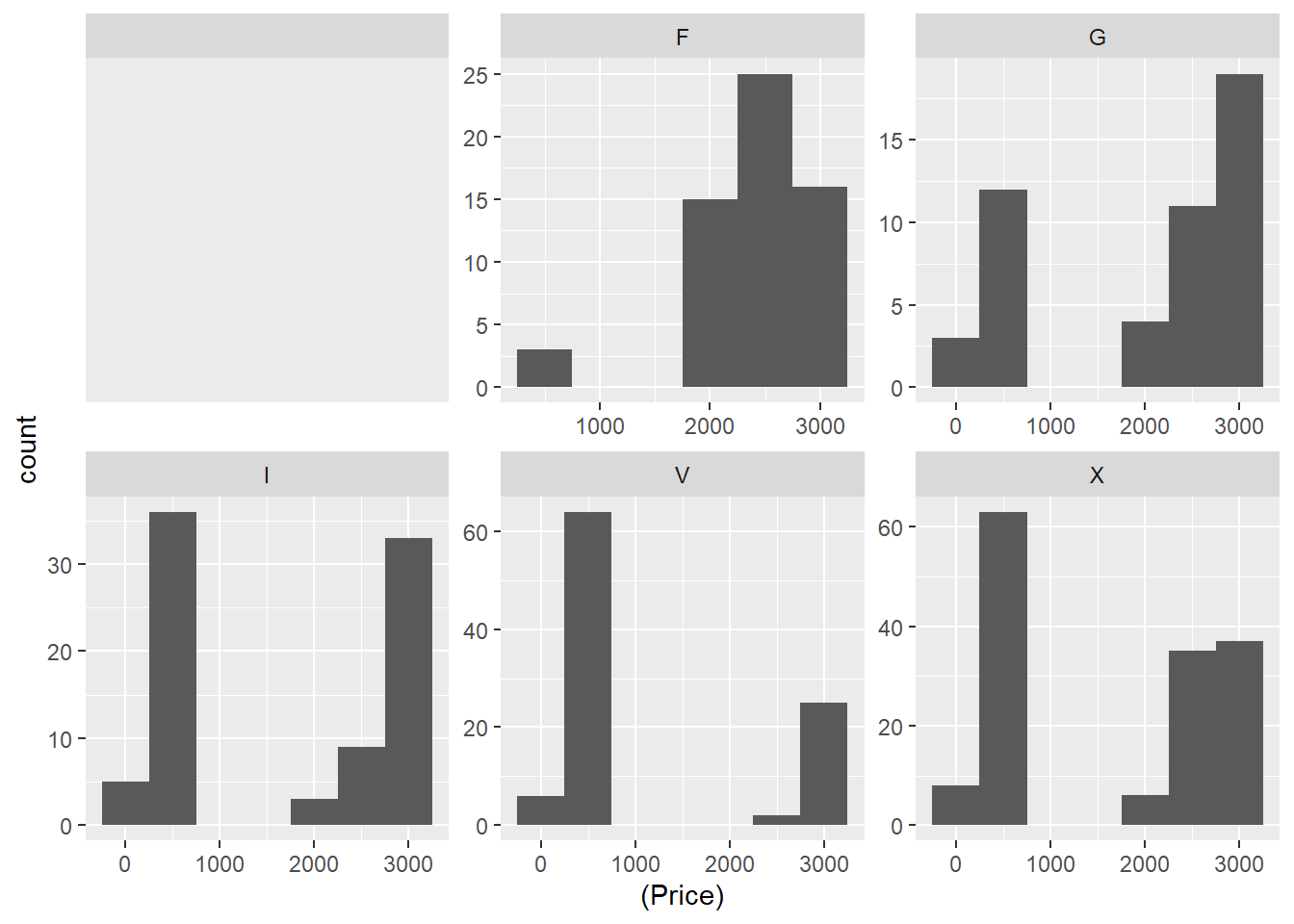
Graphical Display of Data
Histogram of the carat variable:
histogram(~Carat, data=diamonds)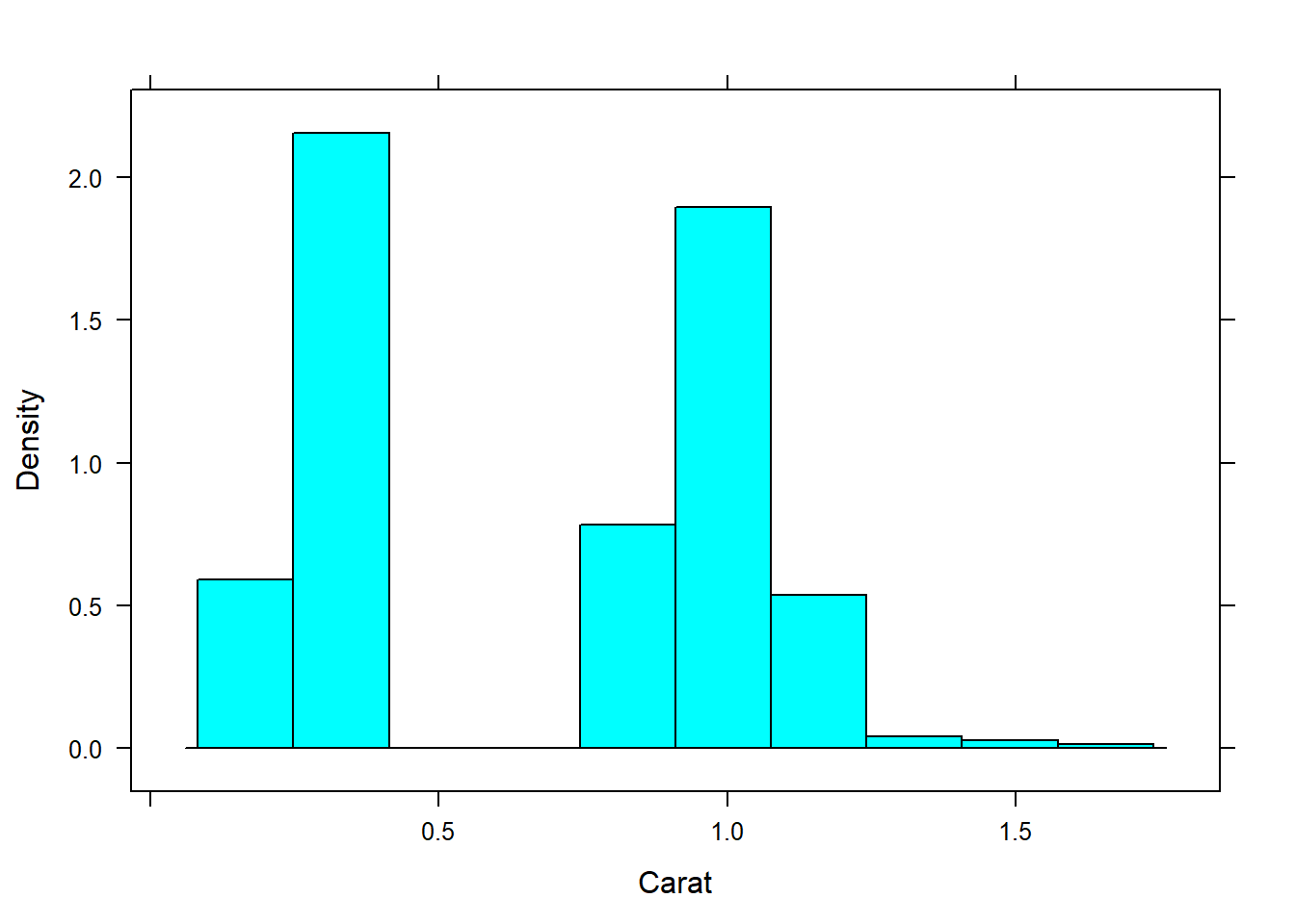
Adjust the binwidth of the histogram:
histogram(~Carat, data=diamonds, width = 0.1)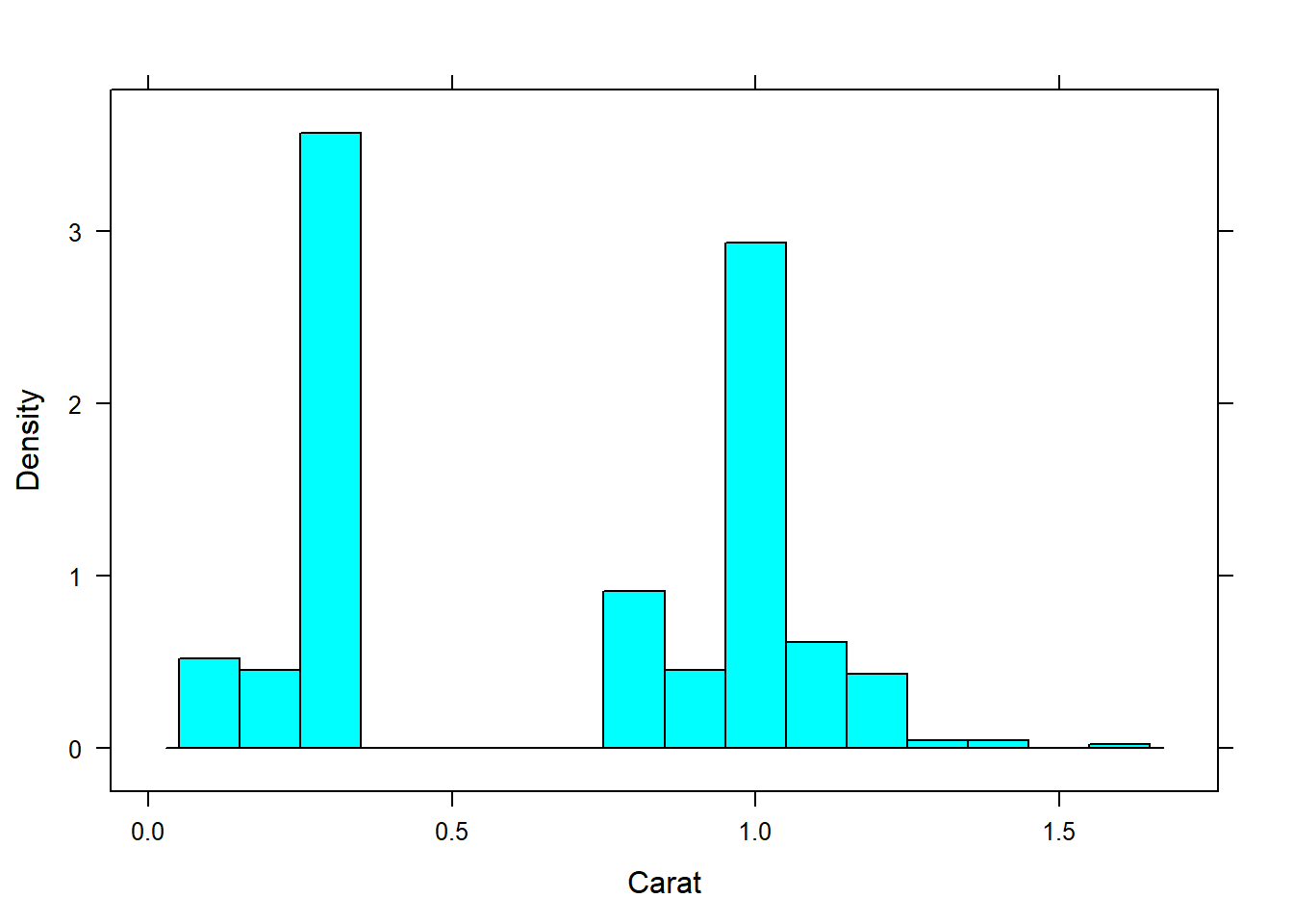
histogram(~Carat, data=diamonds, width = 0.01)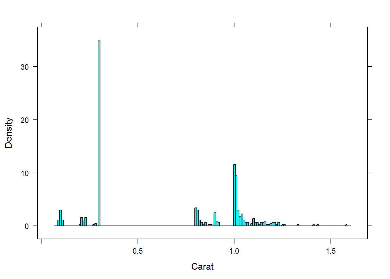
Adjust the number of intervals:
histogram(~Carat, data=diamonds, nint = 50)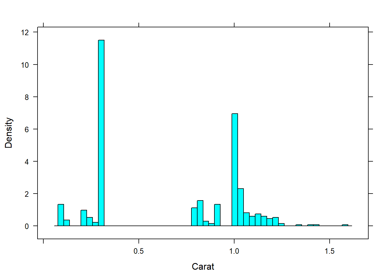 Boxplots:
bwplot(Clarity ~ Price, data=diamonds)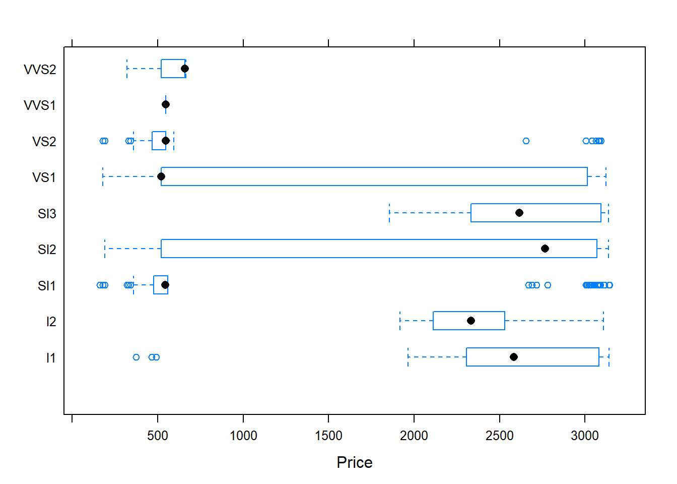
Scatterplots:
Scatterplot between carat and price of diamonds:
qplot(Carat, Price, data=diamonds)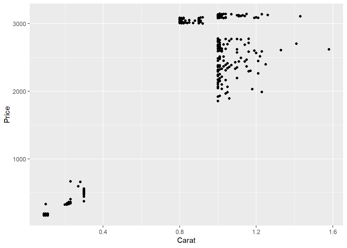
Relationship of Price and Cut
Through a box plot, we observe that the highest price diamonds are premium cut, lowest price diamonds are ideal cut.
dim(diamonds)## [1] 441 9samp_index = sample(1:nrow(diamonds), 30, replace = FALSE) # Creating a random sample to look at the data set.
samp_index## [1] 63 191 10 311 211 213 171 304 403 293 382 369 109 12 96 406 298 192 285
## [20] 116 437 367 132 355 75 161 215 377 425 145diamonds[samp_index,]## Carat Colour Clarity Cut Certification Polish Symmetry Price Wholesaler
## 63 1.00 K I2 F GIA V V 1918 2
## 191 1.01 E I1 X EGL G G 2511 2
## 10 0.80 D SI2 V GIA V X 3012 1
## 311 0.30 I SI1 I GIA V V 493 3
## 211 1.01 I I1 X GIA V G 2651 2
## 213 1.00 L VS2 F GIA G G 2655 2
## 171 1.01 J SI2 I EGL V X 3139 2
## 304 0.30 D I1 X GIA V V 490 3
## 403 0.30 H SI1 X GIA G G 547 3
## 293 0.30 J SI1 G GIA X X 466 3
## 382 0.30 I SI1 I GIA V V 531 3
## 369 0.30 J VS1 V GIA V V 520 3
## 109 1.15 J I1 F EGL G G 2368 2
## 12 0.83 G SI2 I GIA X X 3014 1
## 96 1.00 J SI3 F EGL G G 2310 2
## 406 0.30 H SI1 V GIA X V 547 3
## 298 0.30 I SI2 I GIA X X 476 3
## 192 1.22 K I1 F EGL V G 2516 2
## 285 0.28 E VVS2 X GIA V X 658 3
## 116 1.05 I I1 F GIA G G 2413 2
## 437 0.30 H SI1 G GIA V V 559 3
## 367 0.30 J VS1 V GIA V V 520 3
## 132 1.02 K VS2 I EGL X X 3093 2
## 355 0.30 I SI1 F GIA G V 520 3
## 75 1.00 H SI3 F EGL F F 2101 2
## 161 1.02 I SI3 X EGL G G 3130 2
## 215 1.01 K SI1 F EGL V G 2668 2
## 377 0.30 J VS1 I GIA V V 520 3
## 425 0.30 I VS2 V GIA V V 547 3
## 145 1.01 F SI3 I EGL V G 3111 2str(diamonds$Carat)## num [1:441] 0.92 0.92 0.82 0.81 0.9 0.87 0.8 0.84 0.8 0.8 ...levels(diamonds$Carat)## NULLplot(diamonds$Carat)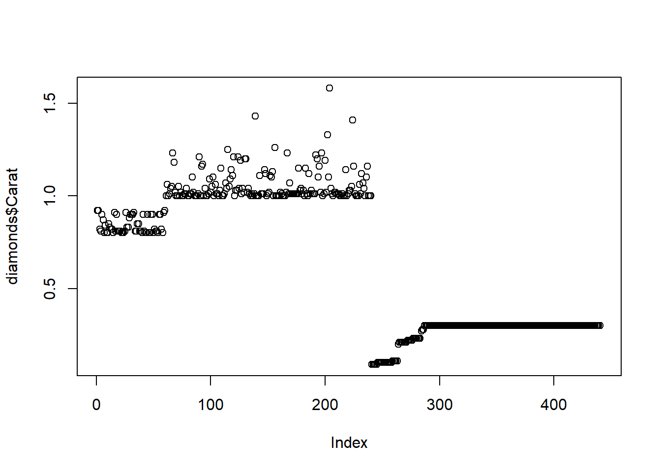
Lets take a closer look at the other ordinal factor variables.
ggplot(diamonds, aes(factor(Cut), Price, fill=Cut)) + geom_boxplot() + ggtitle("Diamond Price according Cut") + xlab("Type of Cut") + ylab("Diamond Price in US Dollars")## Warning: Removed 1 rows containing non-finite values (stat_boxplot).
Price vs Categorical Variables: Clarity, Cut, Color
We can see that these three variables all have a relationship with Price by plotting the categorical variables as colour. We can deduce from this that these three variables are important in predicting price, so we’ll include them as features in our next prediction model.
par(mfrow=c(1,3))
diamonds %>%
  ggplot(aes(log(Price),log(Carat), col= Clarity))+
  geom_point()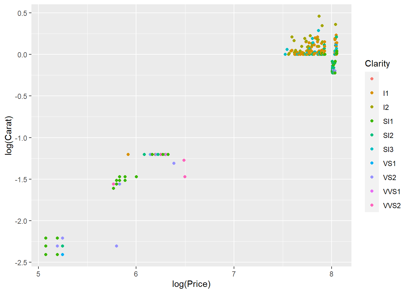
diamonds %>%
  ggplot(aes(log(Price),log(Carat), col= Cut))+
  geom_point()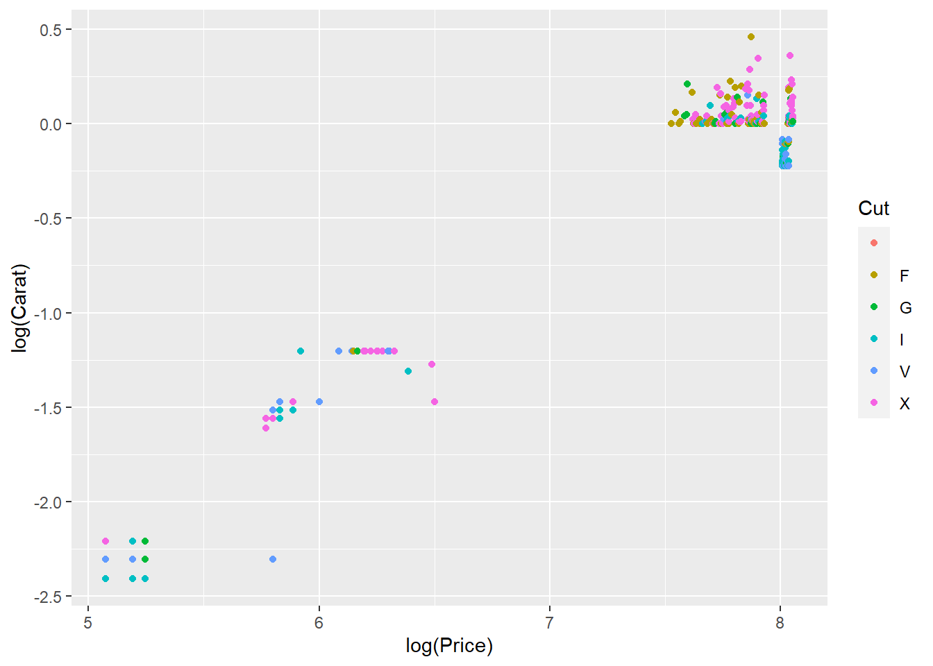
diamonds %>%
  ggplot(aes(log(Price),log(Carat), col= Colour))+
  geom_point()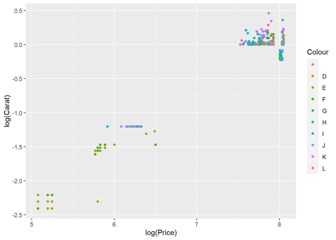
Exploring categorical data
Summarize cuts of diamonds. Since this is a categorical variable we use tables. To create the table, first group by the levels of the cut variable, and then summarize the counts of diamonds in each level.
- Frequency table:
diamonds %>%
  group_by(Cut) %>%
  summarise(counts = n())
## # A tibble: 6 x 2
## Cut counts
## <chr> <int>
## 1 "" 1
## 2 "F" 59
## 3 "G" 49
## 4 "I" 86
## 5 "V" 97
## 6 "X" 149- Proportions table: divide the counts in each level by the number of rows (observations) in the diamonds variable:
diamonds %>%
  group_by(Cut) %>%
  summarise(counts = n() / nrow(diamonds))
## # A tibble: 6 x 2
## Cut counts
## <chr> <dbl>
## 1 "" 0.00227
## 2 "F" 0.134
## 3 "G" 0.111
## 4 "I" 0.195
## 5 "V" 0.220
## 6 "X" 0.338What type of variable is color? Are all colors of diamonds represented in the dataset? Which color is most prominently represented in the dataset?
A useful representation for categorical variables is a bar plot.
ggplot(data = diamonds, aes(x = Colour)) +
  geom_bar()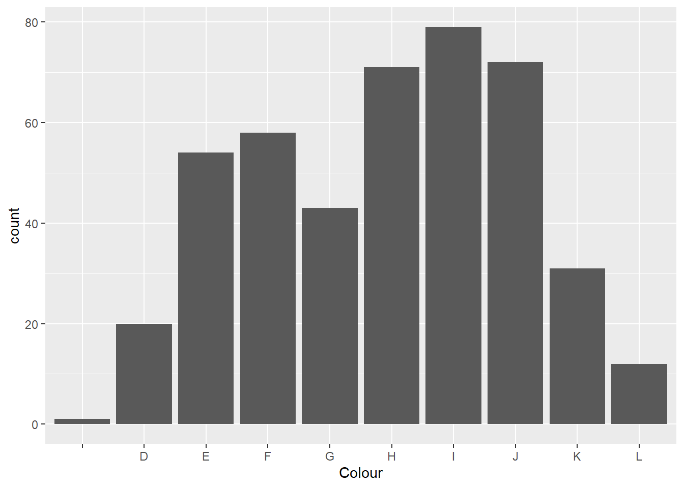
Bivariate Analysis:
We are familiar with the individual variables in the dataset, we can start evaluating relationships between them.
Adding another variable to a histogram:
Let’s make a histogram of the depths of diamonds, with binwidth of 0.2%, and adding another variable i.e cut, to the visualization. We can do this either using an aesthetic or a facet:
- Using aesthetics: Use different colors to fill in for different cuts.
ggplot(data = diamonds, aes(x = Carat, fill = Cut)) +
  geom_histogram(binwidth = 0.2)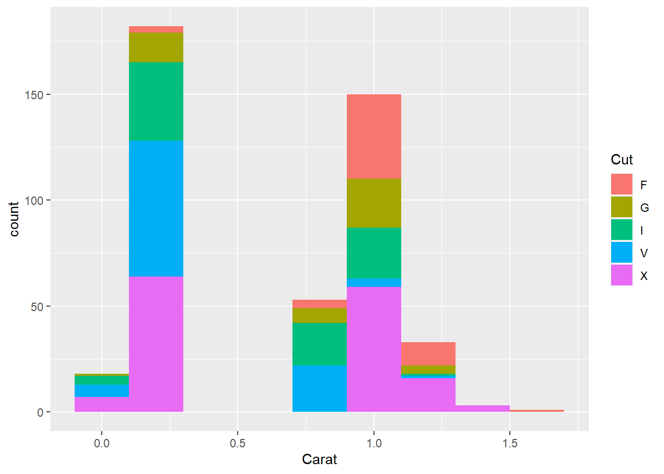
- Using facets: Split into different plots for different cuts.
ggplot(data = diamonds, aes(x = Carat)) +
  geom_histogram(binwidth = 0.2) +
  facet_wrap(~ Cut)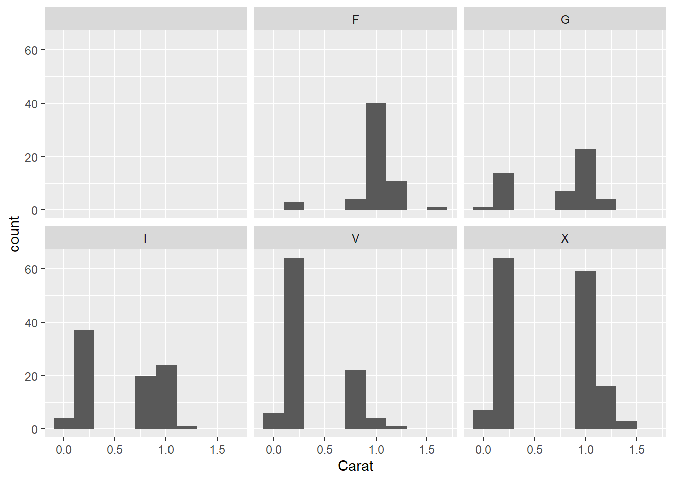
Variable correlated with cut:
Carat and cut have a negative correlation (see box plot below)- fair cuts are typically higher carat, while ideal cuts are typically lower carat. This could be due to the scarcity of larger diamonds, as well as the technical challenge of cutting a large stone into an ideal cut. This is also why lower quality diamonds, even if they are high carats, are more expensive.
diamonds %>%
  ggplot(aes(x=Cut,y=Carat, color=Cut)) +
  geom_boxplot()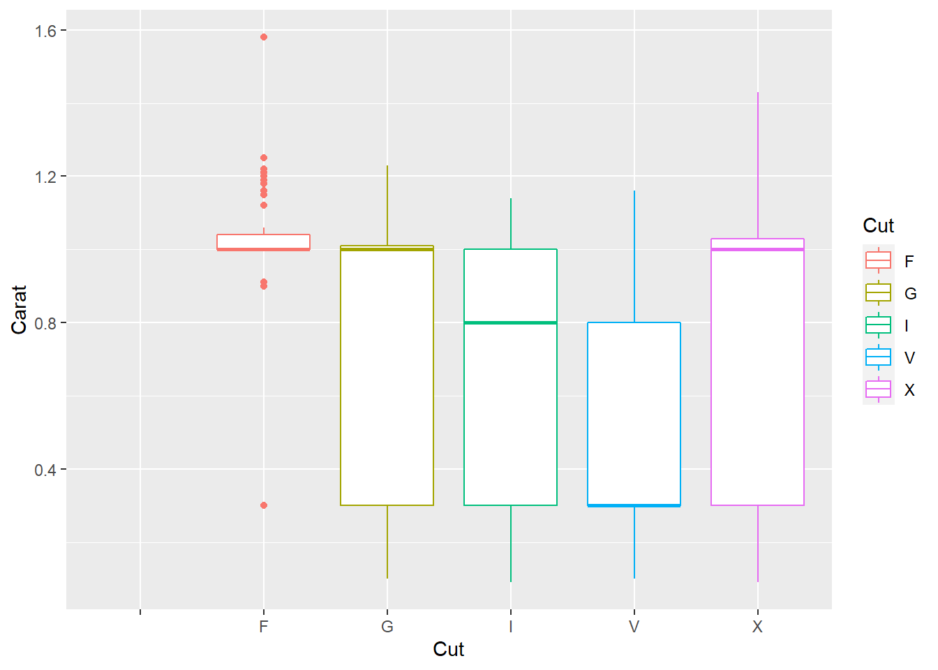
Predicting Diamond Price
To predict diamond price, we would first try to fit the data with a linear regression model.
QQ plot and histogram both show that variable price shows a better normality after log transformation
par(mfrow=c(1,2))
qqnorm((diamonds$Price),main="Normal Q-Q Plot of Price");qqline((diamonds$Price))
qqnorm(log(diamonds$Price),main="Normal Q-Q Plot of log Price");qqline(log(diamonds$Price))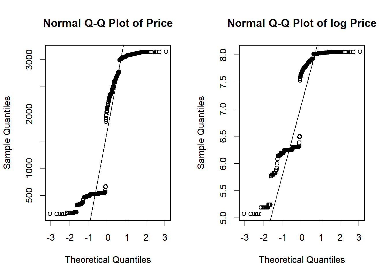
par(mfrow=c(1,2))
hist(diamonds$Price,main="Price")
hist(log(diamonds$Price),main="log Price")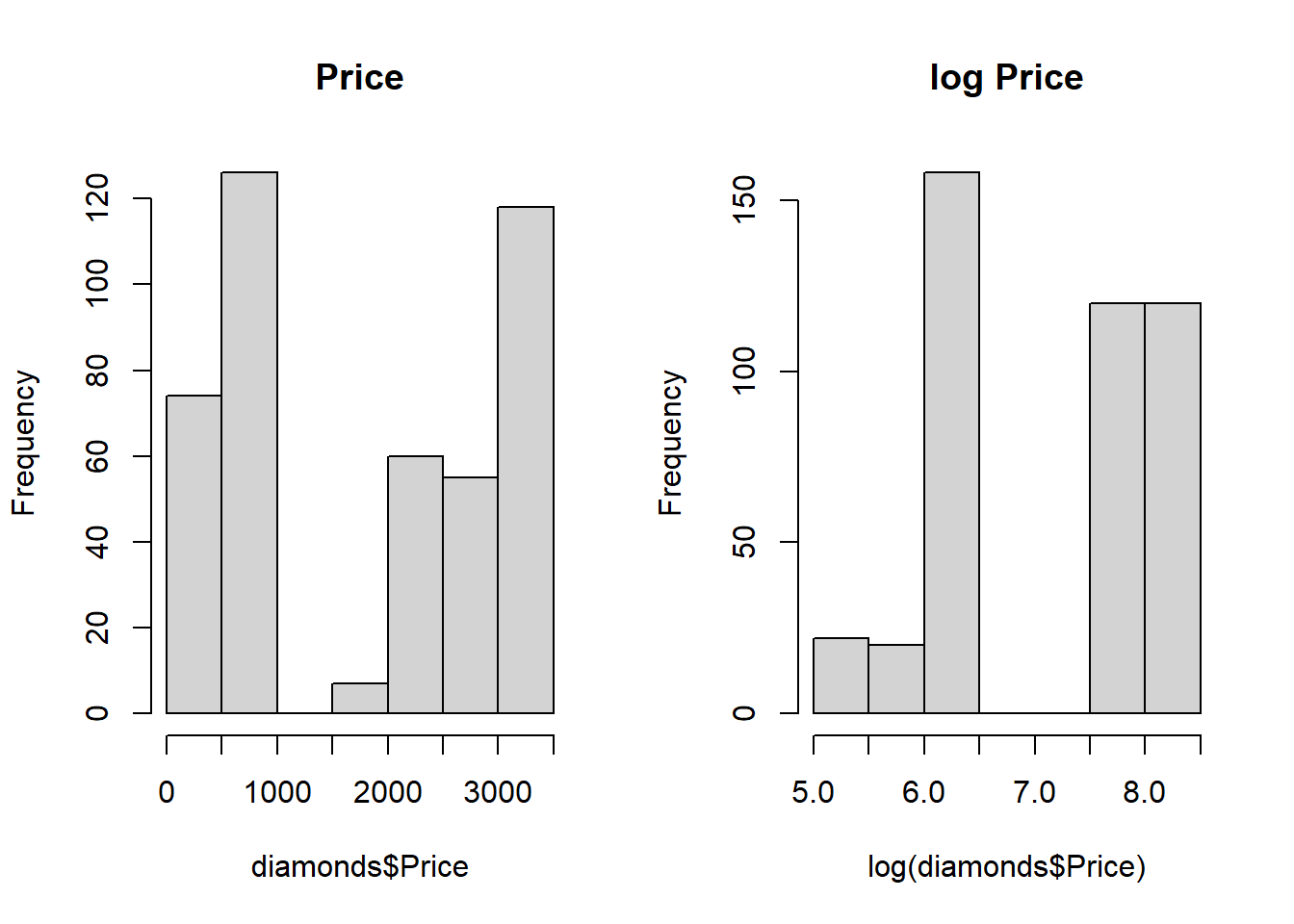
Linear Regression
We use the lm function to build the regression model, with the features that we have selected in earlier sessions.
lm1= lm(log(Price)~ log(Carat) + Cut+Colour+Clarity, data= diamonds)
summary(lm1)
##
## Call:
## lm(formula = log(Price) ~ log(Carat) + Cut + Colour + Clarity,
## data = diamonds)
##
## Residuals:
## Min 1Q Median 3Q Max
## -0.31669 -0.08361 -0.03338 0.07873 0.83362
##
## Coefficients:
## Estimate Std. Error t value Pr(>|t|)
## (Intercept) 7.95244 0.03411 233.162 < 2e-16 ***
## log(Carat) 1.49210 0.01377 108.356 < 2e-16 ***
## CutG 0.02004 0.02676 0.749 0.454312
## CutI 0.04213 0.02464 1.710 0.088033 .
## CutV 0.03127 0.02524 1.239 0.215962
## CutX 0.02768 0.02161 1.281 0.200816
## ColourE -0.02668 0.03545 -0.753 0.452045
## ColourF -0.11124 0.03516 -3.164 0.001671 **
## ColourG -0.13064 0.03618 -3.611 0.000342 ***
## ColourH -0.22083 0.03460 -6.382 4.65e-10 ***
## ColourI -0.26298 0.03455 -7.611 1.82e-13 ***
## ColourJ -0.35873 0.03544 -10.122 < 2e-16 ***
## ColourK -0.39327 0.03996 -9.841 < 2e-16 ***
## ColourL -0.44513 0.05044 -8.825 < 2e-16 ***
## ClarityI2 -0.19748 0.02940 -6.716 6.11e-11 ***
## ClaritySI1 0.37499 0.02641 14.200 < 2e-16 ***
## ClaritySI2 0.29185 0.02197 13.282 < 2e-16 ***
## ClaritySI3 0.09376 0.03107 3.018 0.002701 **
## ClarityVS1 0.51455 0.03576 14.389 < 2e-16 ***
## ClarityVS2 0.44413 0.03275 13.562 < 2e-16 ***
## ClarityVVS1 0.51225 0.10093 5.075 5.83e-07 ***
## ClarityVVS2 0.46022 0.06454 7.131 4.41e-12 ***
## ---
## Signif. codes: 0 '***' 0.001 '**' 0.01 '*' 0.05 '.' 0.1 ' ' 1
##
## Residual standard error: 0.1327 on 418 degrees of freedom
## (1 observation deleted due to missingness)
## Multiple R-squared: 0.9811, Adjusted R-squared: 0.9801
## F-statistic: 1032 on 21 and 418 DF, p-value: < 2.2e-16Compare with a model before log transformation:
lm2= lm(Price~Carat+Cut+Colour+Clarity, data= diamonds)
summary(lm2)
##
## Call:
## lm(formula = Price ~ Carat + Cut + Colour + Clarity, data = diamonds)
##
## Residuals:
## Min 1Q Median 3Q Max
## -871.84 -113.74 -30.85 153.66 758.43
##
## Coefficients:
## Estimate Std. Error t value Pr(>|t|)
## (Intercept) -1262.96 75.10 -16.817 < 2e-16 ***
## Carat 4021.16 47.87 84.007 < 2e-16 ***
## CutG 103.69 45.47 2.280 0.023083 *
## CutI 190.10 41.93 4.533 7.59e-06 ***
## CutV 204.53 43.15 4.740 2.93e-06 ***
## CutX 150.08 36.85 4.073 5.54e-05 ***
## ColourE -222.88 60.13 -3.707 0.000238 ***
## ColourF -326.58 59.66 -5.474 7.59e-08 ***
## ColourG -267.34 61.47 -4.349 1.72e-05 ***
## ColourH -455.52 58.73 -7.756 6.75e-14 ***
## ColourI -512.56 58.61 -8.746 < 2e-16 ***
## ColourJ -729.74 60.22 -12.119 < 2e-16 ***
## ColourK -1004.86 68.61 -14.645 < 2e-16 ***
## ColourL -1138.90 86.13 -13.224 < 2e-16 ***
## ClarityI2 -593.78 50.17 -11.835 < 2e-16 ***
## ClaritySI1 955.49 46.18 20.691 < 2e-16 ***
## ClaritySI2 812.39 38.59 21.052 < 2e-16 ***
## ClaritySI3 236.55 52.83 4.477 9.77e-06 ***
## ClarityVS1 1187.11 61.77 19.219 < 2e-16 ***
## ClarityVS2 1039.77 56.81 18.304 < 2e-16 ***
## ClarityVVS1 1431.16 173.41 8.253 2.04e-15 ***
## ClarityVVS2 1031.59 111.48 9.254 < 2e-16 ***
## ---
## Signif. codes: 0 '***' 0.001 '**' 0.01 '*' 0.05 '.' 0.1 ' ' 1
##
## Residual standard error: 225.5 on 418 degrees of freedom
## (1 observation deleted due to missingness)
## Multiple R-squared: 0.965, Adjusted R-squared: 0.9632
## F-statistic: 548.5 on 21 and 418 DF, p-value: < 2.2e-16The results show that lm1 outperforms lm2; however, while lm2 is adequate, there is a risk of inaccurate estimates from lm2 due to its violation of the regression assumptions. Standardized beta coefficients can be used to determine which feature has the greatest impact on price prediction because the coefficients are all on the same scale:
lm.beta(lm1)## log(Carat) CutG CutI CutV CutX ColourE
## 1.14734123 NA NA NA 0.02128562 NA
## ColourF ColourG ColourH ColourI ColourJ ColourK
## NA NA -0.16980633 NA NA NA
## ColourL ClarityI2 ClaritySI1 ClaritySI2 ClaritySI3 ClarityVS1
## -0.34228223 NA NA NA 0.07209822 NA
## ClarityVS2 ClarityVVS1 ClarityVVS2
## NA NA 0.35388233