pp <- read_csv("paris-paintings.csv", na = c("n/a", "", "NA"))

## 
## -- Column specification --------------------------------------------------------
## cols(
##   .default = col_double(),
##   name = col_character(),
##   sale = col_character(),
##   lot = col_character(),
##   dealer = col_character(),
##   origin_author = col_character(),
##   origin_cat = col_character(),
##   school_pntg = col_character(),
##   price = col_number(),
##   subject = col_character(),
##   authorstandard = col_character(),
##   authorstyle = col_character(),
##   author = col_character(),
##   winningbidder = col_character(),
##   winningbiddertype = col_character(),
##   endbuyer = col_character(),
##   type_intermed = col_character(),
##   Shape = col_character(),
##   material = col_character(),
##   mat = col_character(),
##   materialCat = col_character()
## )
## i Use `spec()` for the full column specifications.

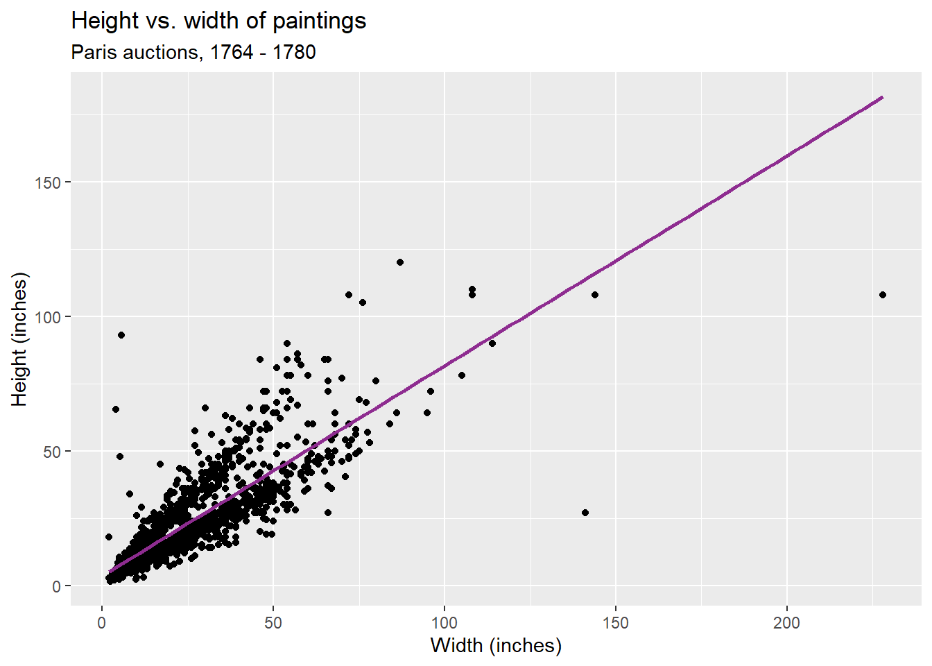
Step 1: Specify model

linear_reg()

## Linear Regression Model Specification (regression)

Step 2: Set model fitting engine

linear_reg() %>%
  set_engine("lm") # lm: linear model

## Linear Regression Model Specification (regression)
## 
## Computational engine: lm

Step 3: Fit model & estimate parameters

linear_reg() %>%
  set_engine("lm") %>%
  fit(Height_in ~ Width_in, data = pp)

## parsnip model object
## 
## Fit time:  21ms 
## 
## Call:
## stats::lm(formula = Height_in ~ Width_in, data = data)
## 
## Coefficients:
## (Intercept)     Width_in  
##      3.6214       0.7808

A tidy look at model output

linear_reg() %>%
  set_engine("lm") %>%
  fit(Height_in ~ Width_in, data = pp) %>%
  tidy()

## # A tibble: 2 x 5
##   term        estimate std.error statistic  p.value
##   <chr>          <dbl>     <dbl>     <dbl>    <dbl>
## 1 (Intercept)    3.62    0.254        14.3 8.82e-45
## 2 Width_in       0.781   0.00950      82.1 0

Visualizing residuals

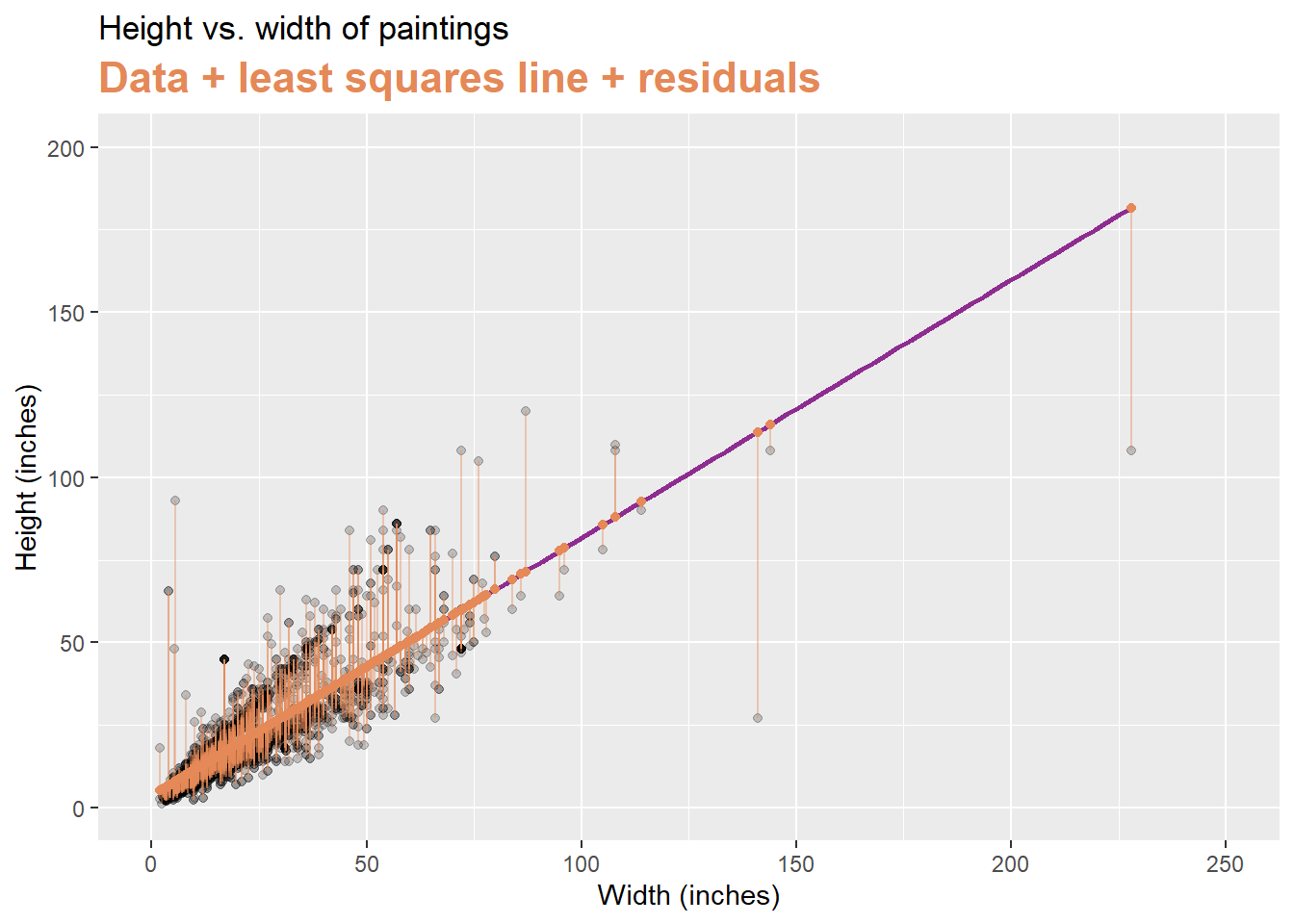
Models with categorical explanatory variables (Height & landscape features)

linear_reg() %>%
  set_engine("lm") %>%
  fit(Height_in ~ factor(landsALL), data = pp) %>%
  tidy()

## # A tibble: 2 x 5
##   term              estimate std.error statistic  p.value
##   <chr>                <dbl>     <dbl>     <dbl>    <dbl>
## 1 (Intercept)          22.7      0.328      69.1 0       
## 2 factor(landsALL)1    -5.65     0.532     -10.6 7.97e-26

#Relationship between height and school

linear_reg() %>%
  set_engine("lm") %>%
  fit(Height_in ~ school_pntg, data = pp) %>%
  tidy()

## # A tibble: 7 x 5
##   term            estimate std.error statistic p.value
##   <chr>              <dbl>     <dbl>     <dbl>   <dbl>
## 1 (Intercept)        14.0       10.0     1.40  0.162  
## 2 school_pntgD/FL     2.33      10.0     0.232 0.816  
## 3 school_pntgF       10.2       10.0     1.02  0.309  
## 4 school_pntgG        1.65      11.9     0.139 0.889  
## 5 school_pntgI       10.3       10.0     1.02  0.306  
## 6 school_pntgS       30.4       11.4     2.68  0.00744
## 7 school_pntgX        2.87      10.3     0.279 0.780

#Categorical predictor with 3+ levels .pull-left-wide[

school_pntg	D_FL	F	G	I	S	X
A	0	0	0	0	0	0
D/FL	1	0	0	0	0	0
F	0	1	0	0	0	0
G	0	0	1	0	0	0
I	0	0	0	1	0	0
S	0	0	0	0	1	0
X	0	0	0	0	0	1

] .pull-right-narrow[ .small[

## # A tibble: 3,393 x 3
##    name      Height_in school_pntg
##    <chr>         <dbl> <chr>      
##  1 L1764-2          37 F          
##  2 L1764-3          18 I          
##  3 L1764-4          13 D/FL       
##  4 L1764-5a         14 F          
##  5 L1764-5b         14 F          
##  6 L1764-6           7 I          
##  7 L1764-7a          6 F          
##  8 L1764-7b          6 F          
##  9 L1764-8          15 I          
## 10 L1764-9a          9 D/FL       
## 11 L1764-9b          9 D/FL       
## 12 L1764-10a        16 X          
## 13 L1764-10b        16 X          
## 14 L1764-10c        16 X          
## 15 L1764-11         20 D/FL       
## 16 L1764-12a        14 D/FL       
## 17 L1764-12b        14 D/FL       
## 18 L1764-13a        15 D/FL       
## 19 L1764-13b        15 D/FL       
## 20 L1764-14         37 F          
## # ... with 3,373 more rows

] ]

---