A03 Assignment EDA1

Jun 4, 2021 · 10 min read ·

Import Lego_sales.csv file

In this assignment we will work with the tidyverse package as usual.We will simulate the data from Lego sales for a sample of customers who bought Legos in the US. The dataset is called lego_sales and is loaded in the data folder.

library(tidyverse)

## -- Attaching packages --------------------------------------- tidyverse 1.3.1 --

## v ggplot2 3.3.3     v purrr   0.3.4
## v tibble  3.1.1     v dplyr   1.0.6
## v tidyr   1.1.3     v stringr 1.4.0
## v readr   1.4.0     v forcats 0.5.1

## -- Conflicts ------------------------------------------ tidyverse_conflicts() --
## x dplyr::filter() masks stats::filter()
## x dplyr::lag()    masks stats::lag()

legosales <- read_csv(file ="lego_sales.csv")

## 
## -- Column specification --------------------------------------------------------
## cols(
##   first_name = col_character(),
##   last_name = col_character(),
##   age = col_double(),
##   phone_number = col_character(),
##   set_id = col_double(),
##   number = col_character(),
##   theme = col_character(),
##   subtheme = col_character(),
##   year = col_double(),
##   name = col_character(),
##   pieces = col_double(),
##   us_price = col_double(),
##   image_url = col_character(),
##   quantity = col_double()
## )

head(legosales)

## # A tibble: 6 x 14
##   first_name last_name   age phone_number set_id number theme    subtheme   year
##   <chr>      <chr>     <dbl> <chr>         <dbl> <chr>  <chr>    <chr>     <dbl>
## 1 Kimberly   Beckstead    24 216-555-2549  24701 76062  DC Comi~ Mighty M~  2018
## 2 Neel       Garvin       35 819-555-3189  25626 70595  Ninjago  Rise of ~  2018
## 3 Neel       Garvin       35 819-555-3189  24665 21031  Archite~ <NA>       2018
## 4 Chelsea    Bouchard     41 <NA>          24695 31048  Creator  <NA>       2018
## 5 Chelsea    Bouchard     41 <NA>          25626 70595  Ninjago  Rise of ~  2018
## 6 Chelsea    Bouchard     41 <NA>          24721 10831  Duplo    <NA>       2018
## # ... with 5 more variables: name <chr>, pieces <dbl>, us_price <dbl>,
## #   image_url <chr>, quantity <dbl>

glimpse(legosales)

## Rows: 620
## Columns: 14
## $ first_name   <chr> "Kimberly", "Neel", "Neel", "Chelsea", "Chelsea", "Chelse~
## $ last_name    <chr> "Beckstead", "Garvin", "Garvin", "Bouchard", "Bouchard", ~
## $ age          <dbl> 24, 35, 35, 41, 41, 41, 19, 19, 37, 37, 19, 19, 20, 36, 3~
## $ phone_number <chr> "216-555-2549", "819-555-3189", "819-555-3189", NA, NA, N~
## $ set_id       <dbl> 24701, 25626, 24665, 24695, 25626, 24721, 24797, 24701, 2~
## $ number       <chr> "76062", "70595", "21031", "31048", "70595", "10831", "75~
## $ theme        <chr> "DC Comics Super Heroes", "Ninjago", "Architecture", "Cre~
## $ subtheme     <chr> "Mighty Micros", "Rise of the Villains", NA, NA, "Rise of~
## $ year         <dbl> 2018, 2018, 2018, 2018, 2018, 2018, 2018, 2018, 2018, 201~
## $ name         <chr> "Robin vs. Bane", "Ultra Stealth Raider", "Burj Khalifa",~
## $ pieces       <dbl> 77, 1093, 333, 368, 1093, 19, 233, 77, 108, NA, 13, 15, 6~
## $ us_price     <dbl> 9.99, 119.99, 39.99, 29.99, 119.99, 9.99, 24.99, 9.99, 9.~
## $ image_url    <chr> "http://images.brickset.com/sets/images/76062-1.jpg", "ht~
## $ quantity     <dbl> 1, 1, 1, 1, 1, 1, 1, 3, 1, 2, 1, 1, 2, 1, 1, 1, 1, 1, 1, ~

Counting frequencies of three most common first names of customers

What are the three most common first names of customers?

Three most common first names of purchasers are Jackson, Jacob and Joseph. Here we count the three most common first names of customers successfully and sort the count in descending order.

library(dplyr)

common_first_names <- legosales %>%
  count(first_name, sort = TRUE) %>%
  top_n(3)%>%
  head(3)
cat("The three most common first names of customers are: ",common_first_names$first_name,sep = "\n ")

## The three most common first names of customers are: 
##  Jackson
##  Jacob
##  Joseph

Three most common themes

What are the three most common themes of lego sets purchased?

Three most common themes of lego sets purchased are Star Wars, Nexo Knights and Mixels. Here we count the three most common themes of lego sets purchased successfully and sort the count in descending order.

common_themes <- legosales %>%
  count(theme, sort = TRUE)  %>%
  top_n(2:3) %>%
  head(3)
  cat("Most common themes are: ",common_themes$theme ,sep = "\n ")

## Most common themes are: 
##  Star Wars
##  Nexo Knights
##  Mixels

Most common subtheme

Among the most common theme of lego sets purchased, what is the most common subtheme?

The most common subtheme among the most common theme of lego sets purchased is The Force Awakens. Here we count the most common subtheme among the common themes of lego sets purchased successfully and sort the count in descending order.

common_subtheme <- legosales %>%
  filter(theme == "Star Wars") %>%
  count(subtheme, sort = TRUE) %>%
  top_n(1) %>%
   head(1)
  cat("The most common subtheme of lego sets purchased is: ",common_subtheme$subtheme ,sep = "\n ")

## The most common subtheme of lego sets purchased is: 
##  The Force Awakens

Creating new variable for age group

Create a new variable called age group and group the ages into the following categories: “18 and under”, “19 - 25”, “26 - 35”, “36 - 50”, “51 and over”.

Here we will create the new variable and called it as age_group. Then group the following categories as:

18 and under
19 - 25
26 - 35
36 - 50
51 and over

    age_group <- legosales %>% 
    mutate(age_group = case_when( age <= 18 ~ "18 and under", 
                                  age >= 19 & age <= 25 ~ "19 - 25", 
                                  age >= 26 & age <= 35 ~ "26 - 35", 
                                  age >= 36 & age <= 50 ~ "36 - 50", 
                                  age >= 51 ~ "51 and over" ))
age_group

## # A tibble: 620 x 15
##    first_name last_name    age phone_number set_id number theme  subtheme   year
##    <chr>      <chr>      <dbl> <chr>         <dbl> <chr>  <chr>  <chr>     <dbl>
##  1 Kimberly   Beckstead     24 216-555-2549  24701 76062  DC Co~ Mighty M~  2018
##  2 Neel       Garvin        35 819-555-3189  25626 70595  Ninja~ Rise of ~  2018
##  3 Neel       Garvin        35 819-555-3189  24665 21031  Archi~ <NA>       2018
##  4 Chelsea    Bouchard      41 <NA>          24695 31048  Creat~ <NA>       2018
##  5 Chelsea    Bouchard      41 <NA>          25626 70595  Ninja~ Rise of ~  2018
##  6 Chelsea    Bouchard      41 <NA>          24721 10831  Duplo  <NA>       2018
##  7 Bryanna    Welsh         19 <NA>          24797 75138  Star ~ Episode V  2018
##  8 Bryanna    Welsh         19 <NA>          24701 76062  DC Co~ Mighty M~  2018
##  9 Caleb      Garcia-Wi~    37 907-555-9236  24730 41115  Frien~ <NA>       2018
## 10 Caleb      Garcia-Wi~    37 907-555-9236  25611 21127  Minec~ Minifig-~  2018
## # ... with 610 more rows, and 6 more variables: name <chr>, pieces <dbl>,
## #   us_price <dbl>, image_url <chr>, quantity <dbl>, age_group <chr>

Probability a randomly selected customer

What is the probability a randomly selected customer?
- is in the 19 - 25 age group?
- is in the 19 - 25 age group and purchased a Duplo theme set?
- is in the 19 - 25 age group given they purchased a Duplo theme set?

Probability a randomly selected customer is in the 19 - 25 age group: It is calculated by dividing the customer in the age group of 19 - 25 by total number of customers in the lego_sales.So, the Probability of a randomly selected customer is in the 19 - 25 age group is 0.2080645.

age_group_19to25 <- age_group %>%
count(age_group) %>%
  filter(age_group=="19 - 25")

probability_19to25 <- (age_group_19to25$n/nrow(legosales)) 
  

cat("Probability of a randomly selected customer is in the 19 - 25 age group: ",probability_19to25 ,sep = "\n ")

## Probability of a randomly selected customer is in the 19 - 25 age group: 
##  0.2080645

Probability a randomly selected customer is in the 19 - 25 age group and purchased a Duplo theme set:

It is calculated by dividing the customer in the age group of 19 - 25 who purchased a Duplo theme set by total number of customers in the lego_sales.So, the Probability a randomly selected customer is in the 19 - 25 age group and purchased a Duplo theme set is 0.01451613.

duplotheme_19to25  <- age_group %>%
  filter( age_group=="19 - 25" & theme=="Duplo")

probability_duplotheme_19to25 <- (nrow(duplotheme_19to25)/nrow(legosales))

cat("Probability a randomly selected customer is in the 19 - 25 age group and purchased a Duplo theme set:",probability_duplotheme_19to25 ,sep = "\n ")

## Probability a randomly selected customer is in the 19 - 25 age group and purchased a Duplo theme set:
##  0.01451613

Probability a randomly selected customer is in the 19 - 25 age group given they purchased a Duplo theme set: It is calculated by dividing the customer of Duplo theme purchaser under the age group of 19 - 25 by total number duplo theme set in the lego_sales.So, the Probability of a randomly selected customer is in the 19 - 25 age group given they purchased a Duplo theme set is 0.2571429.

duplo_theme_set  <- age_group %>%
  filter(theme=="Duplo")
  
probability_duplo_theme <- (nrow(duplotheme_19to25 )/nrow(duplo_theme_set))


cat("Probability of a randomly selected customer is in the 19 - 25 age group given they purchased a Duplo theme set: ",probability_duplo_theme ,sep = "\n ")

## Probability of a randomly selected customer is in the 19 - 25 age group given they purchased a Duplo theme set: 
##  0.2571429

Age group that has spent the largest number of lego sets

Which age group has purchased the largest number of lego sets? How many did they purchase?

Consider the quantity of purchases to check which age group has purchased the largest number of lego sets.So, age group 36-50 has purchased the largest number of lego sets and they purchased 313 total number.

age_group_purchased <- age_group %>% 
  group_by(age_group) %>% 
  summarise(purchase = sum(quantity)) %>% 
  arrange(desc(purchase)) %>%
  head(1)
  cat("The age group has purchased the largest number of lego sets is  ",age_group_purchased$age_group ,sep = "\n ")

## The age group has purchased the largest number of lego sets is  
##  36 - 50

  cat("Total number of lego sets purchased: ",age_group_purchased$purchase,sep="\n")

## Total number of lego sets purchased: 
## 313

Age group that has spent the most money on lego sets

Which age group has spent the most money on legos? How much did they spend?

We need to consider quantity of purchases as well as price of lego sets. So, by analysis it is cleared that age group 36-50 has spent the most money on lego sets and they purchased 9532.87 total_spent.

money_spent <- age_group %>%
 mutate(amount_spent = us_price * quantity) %>%
  group_by(age_group) %>%
  summarise(total_spent = sum(amount_spent)) %>%
  arrange(desc(total_spent)) %>%
  head(1)
  cat("The age group that has spent the most money on Lego sets is:  ",money_spent$age_group ,sep = "\n ")

## The age group that has spent the most money on Lego sets is:  
##  36 - 50

  cat("They spend amount of US dollars equal to  ",money_spent$total_spent ,sep = "\n ")

## They spend amount of US dollars equal to  
##  9532.87

Calculating Theme Name and Median Piece Count

Which Themes have the most Piece Counts associated with it?

To calculate the the most Piece Counts associated with Themes,apply filter to pick only the theme data set, then We group by theme with summarise of MedianPieceCount arranged in descending order.GGplot of theme and MedianPiececount is plotted and it clears that Seasonal,Bionicle, Disney Princess, DC Comics Super Heros and Mixels are the themes which have the most Piece Counts associated with it.

legosales %>%
  filter(!is.na(theme)) %>%
  group_by(theme) %>%
  summarise(MedianPieceCount=median(pieces,na.rm=TRUE)) %>%
  arrange(desc(MedianPieceCount)) %>%
  ungroup() %>%
  mutate(theme = reorder(theme,MedianPieceCount)) %>%
  tail(10) %>%
  
  ggplot(aes(x = theme,y = MedianPieceCount)) +
  geom_bar(stat="identity", color="blue", fill="green") +
  labs(x = 'Theme name', 
       y = 'Median Piece Count', 
       title = 'Theme name and Median Piece Count') +
  coord_flip() +
  theme_bw()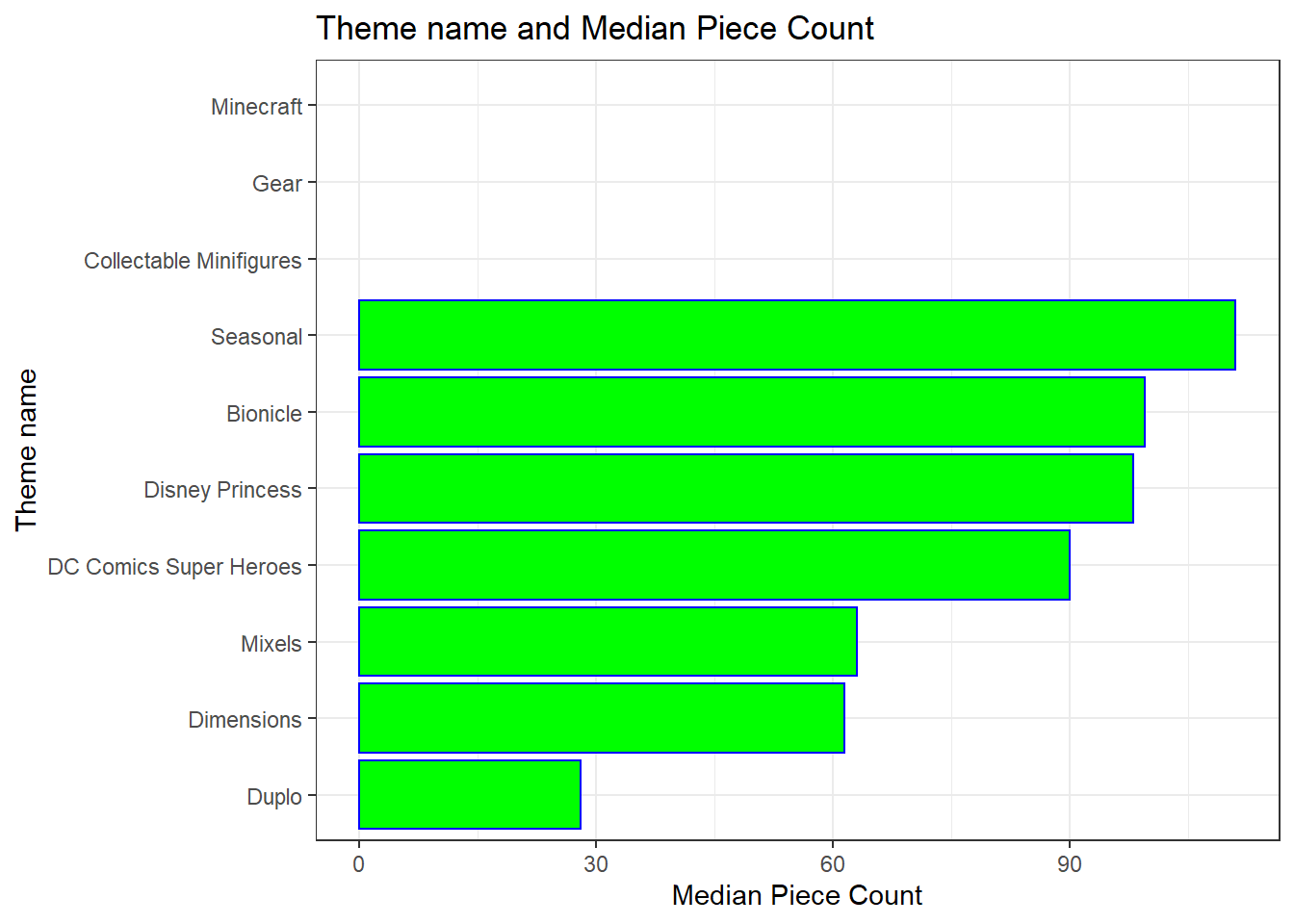

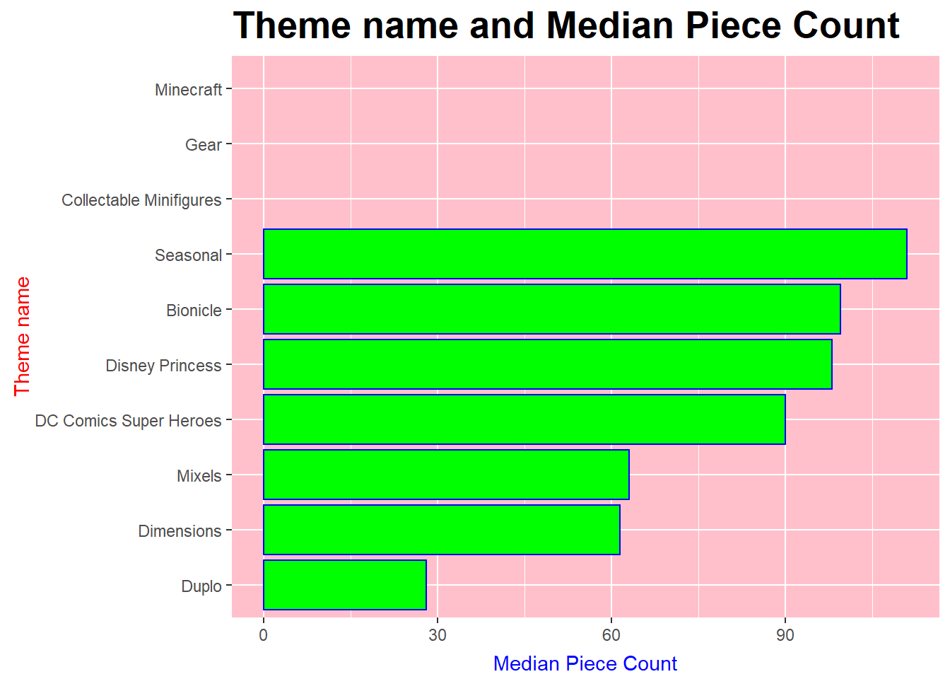
Changing the look of the previous exercise plot without changing the underlying data

Add one element to the plot from the previous exercise to change the look of the plot without changing the underlying data.

The plot shows the change in the following:
- font of title- bold and Bauhaus 93 family used.
- axis title color- x title is blue colored and y axis title is red
- shift in the position of labels of axis - margin is given to the title of axis i.e .35
- panel background color - changed to pink

library(extrafont)
library(tidyverse)
legosales %>%
 filter(!is.na(theme)) %>%
  group_by(theme) %>%
  summarise(MedianPieceCount=median(pieces,na.rm=TRUE)) %>%
  arrange(desc(MedianPieceCount)) %>%
  ungroup() %>%
  mutate(theme = reorder(theme,MedianPieceCount)) %>%
  tail(10) %>%
  
  ggplot(aes(x = theme,y = MedianPieceCount))+
   geom_bar(stat="identity", color="blue", fill="green") +
  labs(x = 'Theme name', 
       y = 'Median Piece Count') +
  theme(axis.title.x = element_text(color="blue", vjust=-0.35),
  axis.title.y = element_text(color="red" , vjust=0.35))+
  ggtitle('Theme name and Median Piece Count')+
  theme(plot.title = element_text(size=20,face="bold",lineheight=.8, 
  vjust=1,family="Bauhaus 93",))+
  theme(panel.background = element_rect(fill = 'pink'))+
  coord_flip()