Assignment A01 based on mtcars dataset
Our analysis will start with the data and then show different links between the car’s design and the miles it can achieve per gallon. Below is a detailed report with our code and methods.
Description:
The data was extracted from the US magazine Motor Trend 1974 and includes fuel consumption and 10 car design and performance aspects for 32 cars (1973-74 models).
Source Data:
We have used the mtcars dataset integrated in R.
Given 32 observations dataframe on eleven (numeric) variables
- mpg - Miles per gallon
- cyl - Number of cylinders
- disp- Displacement (cu.in.)
- hp - Gross horsepower
- drat- Rear axle ratio
- wt - Weight (1000 lbs)
- qsec- 1/4 mile time
- vs - Engine (0 = V-shaped, 1 = straight)
- am - Transmission (0 = automatic, 1 = manual)
- gear- Number of forward gears
- carb- Number of carburetors
look at the structure of the mtcars dataset.
str(mtcars)## 'data.frame': 32 obs. of 11 variables:
## $ mpg : num 21 21 22.8 21.4 18.7 18.1 14.3 24.4 22.8 19.2 ...
## $ cyl : num 6 6 4 6 8 6 8 4 4 6 ...
## $ disp: num 160 160 108 258 360 ...
## $ hp : num 110 110 93 110 175 105 245 62 95 123 ...
## $ drat: num 3.9 3.9 3.85 3.08 3.15 2.76 3.21 3.69 3.92 3.92 ...
## $ wt : num 2.62 2.88 2.32 3.21 3.44 ...
## $ qsec: num 16.5 17 18.6 19.4 17 ...
## $ vs : num 0 0 1 1 0 1 0 1 1 1 ...
## $ am : num 1 1 1 0 0 0 0 0 0 0 ...
## $ gear: num 4 4 4 3 3 3 3 4 4 4 ...
## $ carb: num 4 4 1 1 2 1 4 2 2 4 ...summary(mtcars)## mpg cyl disp hp
## Min. :10.40 Min. :4.000 Min. : 71.1 Min. : 52.0
## 1st Qu.:15.43 1st Qu.:4.000 1st Qu.:120.8 1st Qu.: 96.5
## Median :19.20 Median :6.000 Median :196.3 Median :123.0
## Mean :20.09 Mean :6.188 Mean :230.7 Mean :146.7
## 3rd Qu.:22.80 3rd Qu.:8.000 3rd Qu.:326.0 3rd Qu.:180.0
## Max. :33.90 Max. :8.000 Max. :472.0 Max. :335.0
## drat wt qsec vs
## Min. :2.760 Min. :1.513 Min. :14.50 Min. :0.0000
## 1st Qu.:3.080 1st Qu.:2.581 1st Qu.:16.89 1st Qu.:0.0000
## Median :3.695 Median :3.325 Median :17.71 Median :0.0000
## Mean :3.597 Mean :3.217 Mean :17.85 Mean :0.4375
## 3rd Qu.:3.920 3rd Qu.:3.610 3rd Qu.:18.90 3rd Qu.:1.0000
## Max. :4.930 Max. :5.424 Max. :22.90 Max. :1.0000
## am gear carb
## Min. :0.0000 Min. :3.000 Min. :1.000
## 1st Qu.:0.0000 1st Qu.:3.000 1st Qu.:2.000
## Median :0.0000 Median :4.000 Median :2.000
## Mean :0.4062 Mean :3.688 Mean :2.812
## 3rd Qu.:1.0000 3rd Qu.:4.000 3rd Qu.:4.000
## Max. :1.0000 Max. :5.000 Max. :8.000library(dplyr)
mtcars## mpg cyl disp hp drat wt qsec vs am gear carb
## Mazda RX4 21.0 6 160.0 110 3.90 2.620 16.46 0 1 4 4
## Mazda RX4 Wag 21.0 6 160.0 110 3.90 2.875 17.02 0 1 4 4
## Datsun 710 22.8 4 108.0 93 3.85 2.320 18.61 1 1 4 1
## Hornet 4 Drive 21.4 6 258.0 110 3.08 3.215 19.44 1 0 3 1
## Hornet Sportabout 18.7 8 360.0 175 3.15 3.440 17.02 0 0 3 2
## Valiant 18.1 6 225.0 105 2.76 3.460 20.22 1 0 3 1
## Duster 360 14.3 8 360.0 245 3.21 3.570 15.84 0 0 3 4
## Merc 240D 24.4 4 146.7 62 3.69 3.190 20.00 1 0 4 2
## Merc 230 22.8 4 140.8 95 3.92 3.150 22.90 1 0 4 2
## Merc 280 19.2 6 167.6 123 3.92 3.440 18.30 1 0 4 4
## Merc 280C 17.8 6 167.6 123 3.92 3.440 18.90 1 0 4 4
## Merc 450SE 16.4 8 275.8 180 3.07 4.070 17.40 0 0 3 3
## Merc 450SL 17.3 8 275.8 180 3.07 3.730 17.60 0 0 3 3
## Merc 450SLC 15.2 8 275.8 180 3.07 3.780 18.00 0 0 3 3
## Cadillac Fleetwood 10.4 8 472.0 205 2.93 5.250 17.98 0 0 3 4
## Lincoln Continental 10.4 8 460.0 215 3.00 5.424 17.82 0 0 3 4
## Chrysler Imperial 14.7 8 440.0 230 3.23 5.345 17.42 0 0 3 4
## Fiat 128 32.4 4 78.7 66 4.08 2.200 19.47 1 1 4 1
## Honda Civic 30.4 4 75.7 52 4.93 1.615 18.52 1 1 4 2
## Toyota Corolla 33.9 4 71.1 65 4.22 1.835 19.90 1 1 4 1
## Toyota Corona 21.5 4 120.1 97 3.70 2.465 20.01 1 0 3 1
## Dodge Challenger 15.5 8 318.0 150 2.76 3.520 16.87 0 0 3 2
## AMC Javelin 15.2 8 304.0 150 3.15 3.435 17.30 0 0 3 2
## Camaro Z28 13.3 8 350.0 245 3.73 3.840 15.41 0 0 3 4
## Pontiac Firebird 19.2 8 400.0 175 3.08 3.845 17.05 0 0 3 2
## Fiat X1-9 27.3 4 79.0 66 4.08 1.935 18.90 1 1 4 1
## Porsche 914-2 26.0 4 120.3 91 4.43 2.140 16.70 0 1 5 2
## Lotus Europa 30.4 4 95.1 113 3.77 1.513 16.90 1 1 5 2
## Ford Pantera L 15.8 8 351.0 264 4.22 3.170 14.50 0 1 5 4
## Ferrari Dino 19.7 6 145.0 175 3.62 2.770 15.50 0 1 5 6
## Maserati Bora 15.0 8 301.0 335 3.54 3.570 14.60 0 1 5 8
## Volvo 142E 21.4 4 121.0 109 4.11 2.780 18.60 1 1 4 2Gross Horsepower vs Miles per gallon
The effect of this horsepower number on mpg is shown below. Linear regression is then applied to fit the data in a line. With the linear model method, we use geom smooth.
library(ggplot2)

ggplot(mtcars, aes(x=hp,y=mpg)) +
  geom_point(color="blue") +
  geom_smooth(method = "lm", se = FALSE) +
  labs(title= "Horsepower vs MPG",x="Gross horsepower",y= "Miles per gallon",caption ="Source:Henderson and Velleman (1981), Building multiple regression models interactively. Biometrics, 37, 391–411")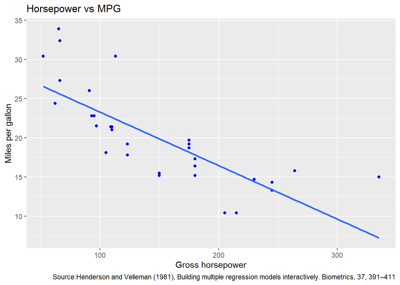
It shows that as the horsepower is increasing,gallon is unlikely to hit zero.
Faceting: individual parts for each vactor level
Impact of Cylinders Number on MPG:
We now carry out the same analysis as above but rather consider the number of cylinders and their effect on gallon(mpg).
library(ggplot2)

plt <-
ggplot(mtcars, aes(x=hp, y=mpg, color=cyl, shape=cyl)) +
    geom_point(size=3) +
   geom_smooth(method="lm", aes(fill=cyl))+
  labs(title= "Facet:Horsepower vs MPG",x="Gross horsepower",y= "Miles per gallon",
       caption ="Source:Henderson and Velleman (1981), Building multiple regression models interactively. Biometrics,37, 391–411")
plt + facet_wrap(~cyl)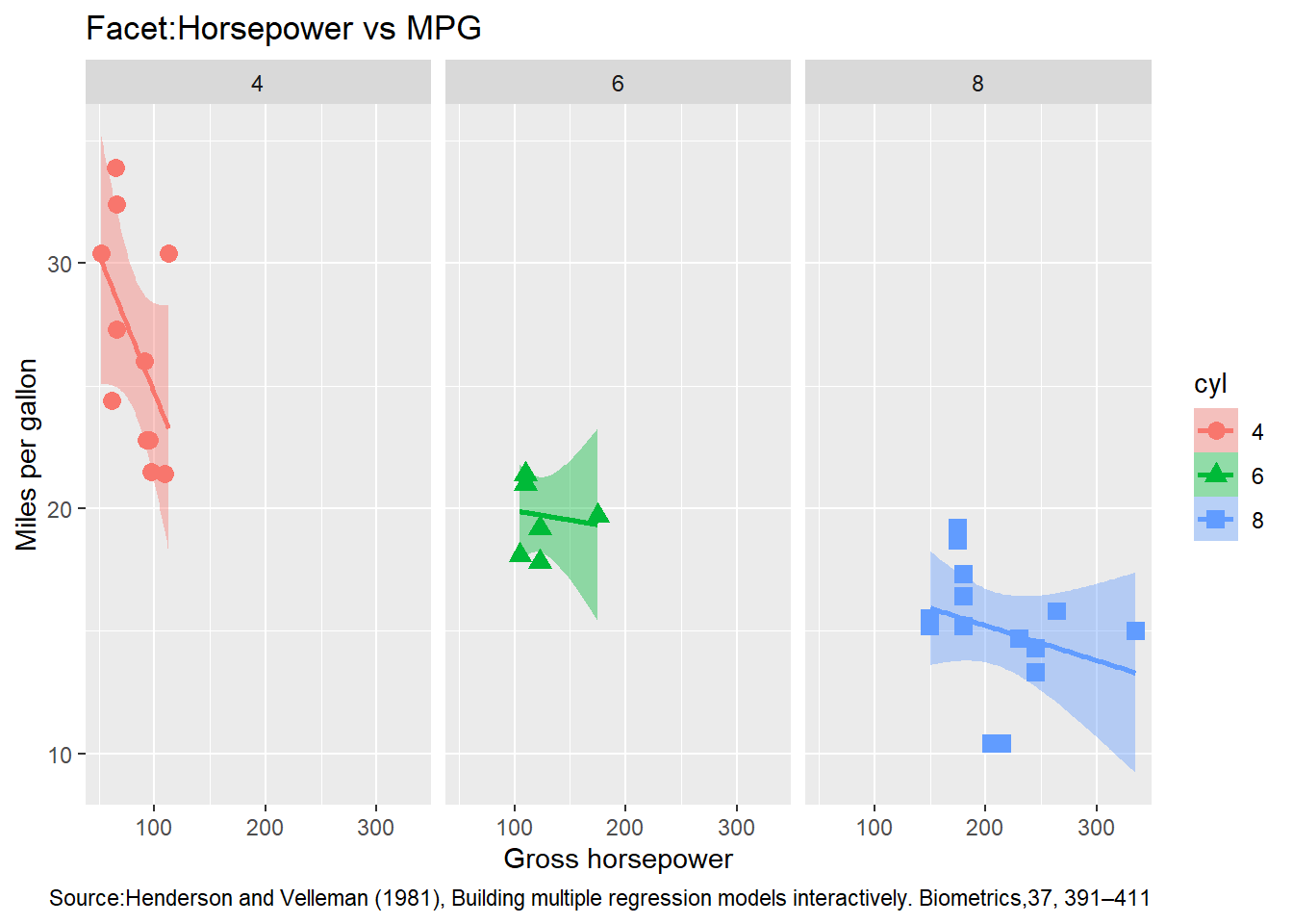
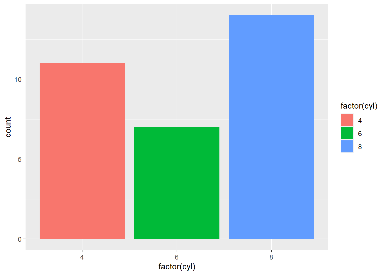
Bar plots
A bar charts is an excellent way to show categorical x-axis variables.
Histograms
To get a sense of how certain data is being analyzed, we compare histograms, first with mpg(miles per gallon) and the second with hp(Gross horsepower).
1: Distribution of Cars by Miles per Gallon
library(ggplot2)

ggplot(mtcars, aes(mpg)) +
  geom_histogram(binwidth = 5) + xlab('Miles per Gallon') + ylab('Number of Cars') +
   ggtitle('Distribution of Cars by Miles per Gallon')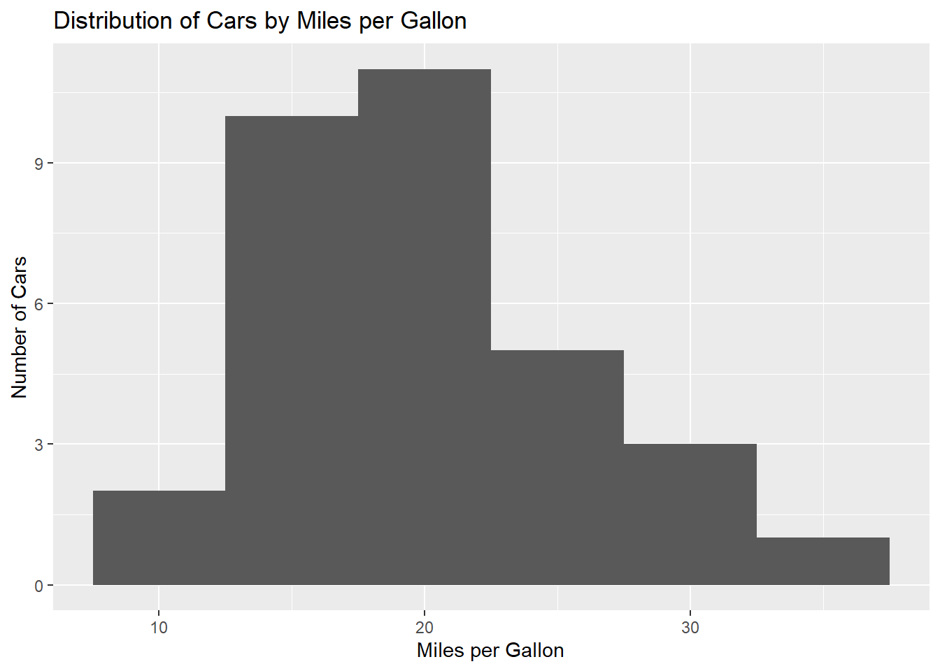
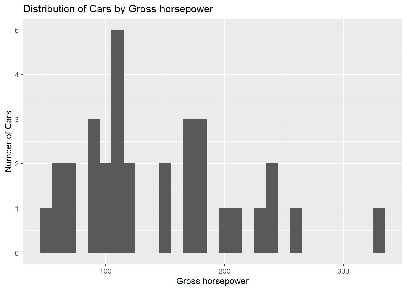
2: Distribution of Cars by Gross horsepower
library(ggplot2)

ggplot(mtcars, aes(hp)) +
  geom_histogram(binwidth=10) + xlab('Gross horsepower') + ylab('Number of Cars') +
  ggtitle('Distribution of Cars by Gross horsepower')